Part 2: Mineral model optimization using a genetic algorithm

I have broken the discussion of genetic algorithms into two posts. The first post focused on the fundamental components of a genetic algorithm (GA) and provided an example. This second post will consist of two main sections. The first section will detail the optimization of the mineral stoichiometry matrix, and the second section will use the optimized stoichiometry as input into a mineral model. I won’t spend a great deal of time dedicated to the Python code, but all the code is available here, or through the link at the bottom of the post.

I guess the first question to address is, why does any of this matter? For the geologist and the petrophysicist, a mineral model is the foundation to other models. If the mineral model is not accurate, then the matrix density is also inaccurate, which leads to error in the porosity and saturation models, and this all feeds into more error in the hydrocarbon-in-place models. Basically, it is a problem of cascading errors, and reducing the error as much as possible in the foundational model is critical. It is also not uncommon to build rock mechanic models based on the mineralogy, especially when sonic log data is absent. And again, error in the mineral model would impact mineral derived acoustic properties, such as Poisson’s ratio and Young’s modulus.

In the modern oil field, these models are then further utilized to build 3D geologic models. The 3D models are then delivered to engineering groups who will use them to aid in completion design and production modeling. By the time the reservoir engineer gets ahold of the output, the error could be significant if care was not taken to build an accurate mineral model.

The problem

What we want to end up with is a model that takes elemental data as input and predicts mineralogy as an output. In this case, 8 minerals will be predicted. The methodology that follows is not the only way that this can be achieved, it is simply one effective method. For instance, my colleague, Randy Blood, uses a pure chemistry and stoichiometry based approach, which also works well.

Portions of this approach were originally detailed by D.D. Eberl in the 2008 USGS publication, User’s Guide to HandLens - A Computer Program that Calculates the Chemistry of Minerals in Mixtures. Eberl’s workflow was originally replicated to closely match the HandLens program, but has since been modified to be suited for optimizing mineral models (instead of chemical formulas).

Assuming a geologist has cuttings, or better yet, core, then they more than likely have collected mineralogy data in the form of X-ray diffraction (XRD). In most cases elemental data has also been collected from X-ray fluorescence (XRF). In these cases, where mineral and elemental data are available on the same sample splits, we can use the two data sets to define the most likely mineral formulas. Once these formulas have been defined, only the elemental data (XRF) is needed for predicting mineralogy in future wells. This is ideal as XRF data can be run on cuttings and is relatively cheap. Alternatively, you can also use elemetal log data (e.g. Schlumberger’s Lithoscanner) as the elemental input. This workflow has been depicted in the high budget graphic below.

Graphical representation of the primary steps from raw sample to final mineral formulas.

This does not provide a totally satisfactory solution. Most oil and gas companies have an abundance of triple-combo log data that they’d prefer to leverage. It is not realistic to expect a full suite of elemental data on all cuttings from all wells. However, a model can be built that utilizes a subset of wells with elemental data to predict mineralogy. This predicted mineralogy, which is a model, could then be used as input to calibrate a triple-combo based mineral model (again, cascading error problem). It is unlikely that a triple-combo model would yield the same number of mineral predictions, but if only the major mineral groups were of importance, such as tectosilicates, phyllosilicates, and carbonates, then it would be effective. This step won’t be covered in this post because the current dataset is limited.

Section 1 - Optimization

Geologists work in the realm of uncertainty and this is often reflected in the analyses they provide. This uncertainty can be frustrating to their engineering colleagues, but it is just the reality of the available data. Tuning, or more appropriately, optimization, is one way to help reduce the uncertainty. A perfect solution can not be provided, but a solution that leverages your available data can be. Genetic algorithms are not the only optimization method, but they are effective, and will be utilized here.

There is a bit of care that must be taken when defining the target function when building an optimization workflow. Specifically, we must utilize a function that can determine if the GA is improving, we need something to act as a fitness metric. For this particular problem, we are using elemental data, elemental fractions, and mineral data. The elemental and mineral data are given, but the elemental fractions are unknown. These fractions are what need to be optimized. Listed below are the data and the primary math steps:

e = one vector entry per sample of elemental data, percent values (XRF, known)

m = one vector entry per sample of mineral data, weight percent values (XRD, known)

F = matrix of elemental fractions (unknown)

We also know that the elemental abundance should be controlled by the minerals that are present and how much of each element is in each mineral. This leads to the following relationship:

However, we don’t need to solve for e, we need to solve for m, and since this is a linear algebra problem, that means that we need to take the inverse of F, (F^-1):

Eqn. 2 is not the target function, but it provides the necessary input for the target function, specifically the m prediction, which will be depicted as m-hat below. The target function will be a minimization of the residual sum of squares (rss), which is further summed over all samples:

One thing to point out about using rss as a fitness metric is that it will preferentially “favor” the minerals that are in higher abundance, at least in the earlier generations. This is due to the fact that correcting the error on the higher abundance minerals serves to more effectively reduce rss.

The following is debatably a distraction, but there is at least one alternative that will be used as a fitness metric, and that is the root relative square error (rrse). Using rrse would normalize each mineral’s error relative to its variance, which would essentially put low-abundance and high-abundance minerals on the same playing field. Both fitness metrics have been used to build an optimized F matrix, and the resulting mineral models for both can be compared, which will be included in Section 2.

Shown below is the alternate target function using root relative square error:

In words, what the rrse function is doing, is comparing the model performance to a simple model, which is just the average. This is done for each mineral and summed over all samples. Finally, since 8 minerals are evaluated, but a single target value is needed, the average rrse for all minerals is reported, which is shown as the summation from i to n multiplied by 1/n outside the square root.

One interesting point to make regarding the rrse metric is that, as the name implies, it is a relative metric, and it is relative to the performance of a simple model, m-bar. This implies the following:

rrse = 1: the model error is equal to that of a simple model

0 < rrse < 1: the model error is less than a simple model

rrse >1: the model error is greater than a simple model

rrse = 0: the model is perfect and has zero error (rrse can’t be less than 0)

Therefore, a low rrse value that approaches zero is desired. A value close to 1 or greater than 1 indicates we may have been better off saving ourselves all the trouble and just using the average.

The data

A number of matrices have been discussed, but it is probably a good idea to have a look at each of these. The data that is being used for this analysis came from three different wells and covers several lithology types. In total there are 75 samples, but 21 of the samples are being retained as a blind.

The blind samples all come from the same well, which generally tends to lead to an increase in the blind error, as opposed to a blind that is randomly withheld from all of the data. This is due to the fact that when some samples from all the wells are used as the blind, the model gets to “see” samples from each well in the training set, but when an entire well is retained as the blind, the model is tested against completely new data. This is important because data from different wells often introduces new variance to the dataset via geologic variance, vendor variance, and/or vintage variance. If a model shows low error on a blind well, despite the possibility of new variance, then this implies better generalization of the model.

Elemental Data (e)

As can be seen above, not all of the elemental data from the XRF is utilized, but the major elements are included. The ‘Unity’ column adds one more equation to the linear system, and is included under the assumption that the sum of all the minerals being modeled is equal to 100%. This assumption is not true, but it is generally reasonable.

Mineral Data (m)

The mineralogy data is in weight percent and includes the primary minerals that compose the lithology of interest. These minerals have been normalized to 100%, so the values are not identical to the actual data. Although this matrix has been normalized, it is still treated as the true or actual values that our predictions (m-hat) will be evaluated against.

Elemental Fractions (F)

The F matrix is a square 8x8 matrix, and is the final output of the optimization process. Each row represents a single mineral and each column is the elemental fraction that is present in the mineral. For example, the calcite (Cal) in row 1 shows about 0.40 calcium (Ca). This indicates that the Ca accounts for 40% of the atomic mass of the calcite mineral. There is also a very small amount of Mg, but it is essentially zero.

The complete mineral formula is not included, which is again apparent using calcite as an example. The chemical formula of calcite is CaCO3, but the carbonate molecule is not included (CO3) in this matrix. Technically, it is included when determining the minimum and maximum allowable fractions for each element in each mineral, but it is excluded here because it is fixed (i.e. it can’t be optimized).

It is also important to point out that minerals like quartz (Qtz - SiO2) have fixed stoichiometry and can’t be optimized, but must be included because they account for a large portion of the Si “consumption”.

GA code discussion

Before getting into the model performance, it is worth briefly summarizing the GA workflow, which was covered in a bit more detail in the previous post. The objective of the problem is the optimization of the F matrix. The GA steps that are to be followed and coded are:

Initial population (generation 1)
Fitness
Crossover
Mutation
Generation 2
Repeat

Initial population (generation 1)

The first generation is the starting point or initiation of the GA. This simply involves making a bunch of guesses for the elemental fractions, and these guesses will be constrained by the stoichiometry. So, depending on which hyper parameters are used (discussed below), our starting generation will be a population of 150 or 200 F matrices, and that’s what is needed to kick things off.

Fitness

As was described in the previous post, the initial fitness of the population as a whole will be poor. But there will be a few parents that are slightly more fit and they will be the ones with the lowest rss or rrse, depending on the fitness metric selected. Much like what was done in the previous post, we can rank the parents from most to least fit, and take the top half.

Since two fitness metrics are being used in the optimization (rss and rrse), we will have two separate optimized F matrices, resulting in two final mineral models.

Crossover

This step gets just a little bit weird. The F matrix is 8x8 in this workflow, and selecting a crossover point within a matrix is an odd concept. Therefore, to make things easy, we can flatten the matrix. First we will drop the unity column, because that never changes, which makes it an 8x7 matrix. The resulting flat matrix is now 1x56 and is essentially a list of numbers that can crossover easily. The matrix just has to be reshaped back into an 8x8 later (8th column coming from the unity column).

The graphic below depicts the matrix flattening using a 3x3 matrix for explanatory purposes, but the process is identical for an 8x8 matrix.

Example 3x3 matrix showing how a matrix is organized after flattening.

Mutation

Mutation is performed on some subset of the genes within a population and is critical for introducing new variance to the population. For this problem there are 56 genes that are available for mutation. As an example, if there are 100 parents in a population and each parent has 56 genes, then there are 5600 possible genes in a given population available for mutation. Using a mutation rate of 2% would lead to 112 possible mutations in a given generation (5600 * 0.02 = 112).

So, in slightly more specific terms, the steps are as follows:

Build a population of F matrices, where each F matrix in the population is essentially an individual parent. This initial population will contain F matrices that are a bunch of random guesses, but the guesses will honor the acceptable ranges of stoichiometry for each mineral. The first population of F matrices represents generation 1.
Make a prediction of the mineralogy (m-hat), using eqn. 2, for each F matrix in the population.
Evaluate the mineral predictions (m-hat) against the actual mineral values (m) using eqn. 3 (rss) or eqn. 4 (rrse). This implies that each F matrix in generation 1 will have a fitness value. If there were 100 parents (F matrices) in generation 1, then there would be 100 fitness values. The F matrices with the lowest error are the ones with highest fitness and will be preferentially carried to generation 2 as the new parents.
Using the most fit parents, apply crossover and mutation to generate new offspring. (note: crossover and mutation were described in the previous post).
Repeat steps 1-4 until error stabilizes.

Graphical representation of the primary steps for optimizing the F matrix.

Hyper tuning

Hyper tuning is the process of systematically altering the settings (parameters) of an algorithm to determine the specific recipe that yields the best results. This step would be completed prior to optimization. For the GA algorithm that has been coded, there are two parameters that need to be evaluated: population size and mutation rate. Obviously the total count of generations will have an impact, but generally, the algorithm will be run for a few more generations than are necessary to ensure that optimization has been achieved. So really what needs to be known are the proper population size and mutation rate that tends to yield the best results.

The sklearn Python library has a great grid search package called GridSearchCV, which is intended for the tuning of hyper parameters. I probably should have used this package, but I decided to build a custom grid search. The grid search allowed the GA to cycle through the following parameters:

population_size = [50, 100, 150, 200, 250]
mutation_rate = [0%, 1%, 2%, 4%, 6%]

Population size refers to the number of F matrices (parents or chromosomes) in each generation. Mutation rate is a percentage of the genes (not parents) that are randomly modified in each generation. Using a mutation percentage, as is shown above, allows the number of mutations to scale appropriately with the changing population size.

There are a total of 25 permutations that need to be tested by the grid search, which is a pretty small space to explore. However, since k-fold cross validation is being used, the run time will be extended. The ‘k’ in k-fold is an indication of how many groups the training data will be broken into. In this workflow, 5 groups were used (k=5) for the cross validation, and this was only applied to the training data, the blind data was not included. The average fitness of the test group will be used to determine the ideal parameter settings.

To (unfortunately) further complicate the matter, the cross validation step was applied using both the rss and rrse fitness metrics. This may have been a step too much, but I was curious to see how impactful a different fitness metric would be on both the hyper parameters and on the mineral model.

Population and mutation optimization using rss as the fitness metric. The optimized grid search solution is shown in blue.

The above plot shows the results of the grid search with cross validation, performed using rss as the fitness metric. The categories shown on the x-axis are all the scenarios investigated by the grid search. A category of “100_2%” indicates that the population size in each generation contained 100 parents and that the mutation rate was 2%. There are two primary take-aways from this plot:

Cases with 0% mutation show poor performance, which is not surprising.
Nearly all the scenarios with any mutation > 0% show similar performance.

In order to really see the difference in the various scenarios, two changes need to be made to the plot above, which are excluding the 0% mutation cases, and constraining the y-axis, shown below.

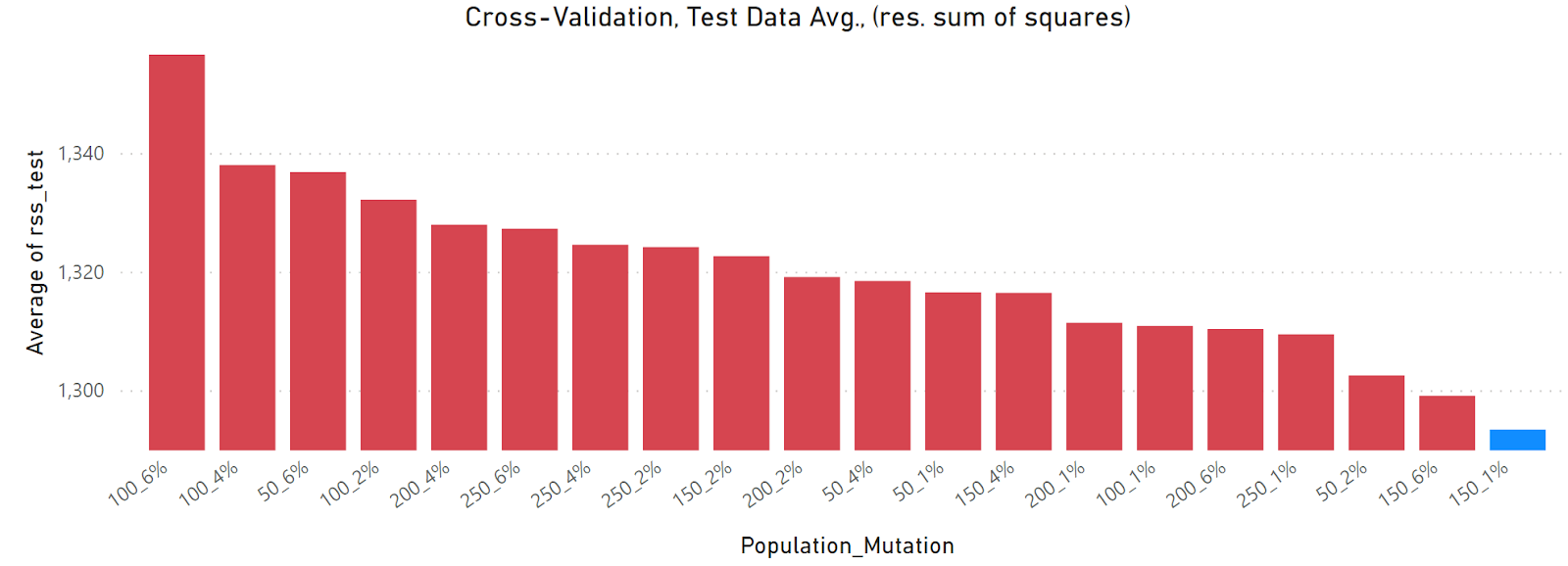
Same as previous image, but with removal of 0% mutation cases and rescaling of the y-axis. The optimized grid search solution is shown in blue.

It’s now easier to see that the best case is a population of 150 and a mutation rate of 1% (shown in blue), but most of the cases are similar and would likely yield comparable models.

The exact exercise that was employed above for the rss fitness metric, can also be repeated, but using rrse as the fitness metric. In this case, only the plot that filters out the 0% mutation and constrains the y-axis will be shown. When rrse is used as the fitness function the results are similar, but in this case a population of 200 and mutation rate of 1% were identified as the optimum hyper parameters (shown below).

Population and mutation optimization using rrse as the fitness metric. The y-axis has been rescaled and the 0% mutation cases have been removed. The optimized grid search solution is shown in blue.

At this point there are two mineral models that can be built, the first model honors the optimization parameters from the rss grid search, and the second honors the optimization parameters from the rrse grid search.

Section 2: Mineral Model

At this point we’ve used a grid search to determine the ideal population size and mutation rate. We then optimized the F matrix using two different fitness functions and the ideal hyper parameters. Now, using our F matrices we can predict mineralogy using elemental data as input. We can generate a few key visualizations, which include:

A. Sample plots showing predicted and actual mineral weight percent for each mineral

B. Cross plots of the predicted vs actual mineral weight percent for each mineral

C. Error tables for minerals using rss and rrse

D. Same as ‘A’, but for the 3 primary mineral groups (tectosilicates, phyllosilicates, carbonates)

E. Same as ‘B’, but for the 3 primary mineral groups (tectosilicates, phyllosilicates, carbonates)

F. Same as ‘C’, but for the 3 primary mineral groups (tectosilicates, phyllosilicates, carbonates)

G. F matrix variance.

For all the plots, the rss, rrse, and r-square will be reported in the error tables. It is also interesting to compare the variance in the optimized F matrix, which is what ‘G’ refers to. For instance, if we were to run the script some set number of times, would we find that the resulting F matrices are essentially the same, and produce nearly identical mineral models, or are widely variable models produced? If the solution is stable, then the expectation would be that the resulting F matrix would have low variance from one trial to the next. In other words, do we always see that the chlorite mineral, for example, has the same optimized fraction of Al and Fe in its chemical composition?

A. Sample Plots (by mineral)

Because there are a total of 8 minerals that are being modeled, there are 8 plots below, one for each mineral. The topmost plot shows the resulting quartz model using rss (red) and rrse (yellow) as the target functions. The blue curve is always the true mineral value from XRD data (blue=true). In these plots, both the training and blind data are shown together, but the blind data can be observed by reviewing the data in sample numbers 14-34 inclusive. Error is not reported in this section, but Section ‘C’, below, will review the error.

Quartz, illite, and calcite are the most abundant minerals and account for about 80% of the total mineralogy. Both mineral models do a good job of predicting these three major minerals, but have trouble with the minerals that are in low abundance (2-4% on average), which would be the bottom 4 plots (pyrite, plagioclase, chlorite, and mixed illite/smectite).

True (blue) vs modeled minerals. The red curve represents the rss based model and the yellow represents the rrse based model.

The plots below the calcite plot indicate that the model starts having some trouble. It follows the general trends, and on average it is very close, but it certainly misses on a number of data points. This downfall is even more apparent when viewing the cross plots further below.

This error would be problematic if your objective as a geologist was to map subtle changes in specific (low-abundance) minerals. However, if the objective was to derive a reasonable grain density, then in most cases, the 4 models below would perform better than a simple model (that is, better than just using the mean).

Continuation of the previous plots, but showing the low-abundance minerals.

B. Cross plots (by mineral)

Before getting into the specific error associated with each model, it is helpful to view the crossplots below. Each plot shows the modeled mineral on the x-axis and the true mineral on the y-axis. Also, please note that the scale changes from one plot to the next. The first 8 crossplots are shown in red and are the result of using rss as the fitness metric. The second 8 crossplots are shown in yellow, and are derived from rrse as the fitness metric. In all the plots below, the black dots are the blind samples.

Cross-Plots: Residual Sum of Squares (rss)

As was seen in the above section, the major minerals like quartz, illite, calcite, which account for about 80% of the bulk mineralogy, show a tight correlation between model and true values. However, the error becomes apparent for the low abundance minerals. As was stated above, the trends are reasonable, but the scatter is fairly high. Mixed illite/smectite is especially poor, but this is in no small part due to the outlier that shows nearly 30% abundance. This data point is likely not accurate as it is off trend with the lithologies in this area, but I was hesitant to remove it until further analysis.

The error tables below show that the r-square for the low-abundance minerals is poor, but the mean absolute error is generally less than that of the higher-abundance minerals. The problem is of course due to the fact that when a mineral is of low abundance, then even a small amount of absolute error can strongly impact the r-square.

Cross-plots by mineral using rss as the fitness metric.

Cross-Plots: Root Relative Square Error (rrse)

The story is basically the same when using the rrse derived mineral model. It’s actually slightly better than the rss model. In full disclosure, I expected the opposite to be the case, that the rss model would be better. I had hypothesized that since the rss model would preferentially correct for the most abundant minerals, that it would result in a better overall model. However, it appears that even though the rrse approach puts the minerals on a more equal playing field, this did not harm its ability to account for the high-abundance minerals.

Cross-plots by mineral using rrse as the fitness metric.

C. Error tables

The visualizations above are certainly helpful for a qualitative understanding of the model error. They are also helpful for determining which minerals are causing the most trouble. However, some actual numbers that address error are necessary to fully describe the model. The two error tables below include a number of metrics that are typically used to assess model accuracy and/or model error. The first table shows the metrics associated with the rss fitness function, and the second with the rrse fitness function. In both cases the blue column is meant to highlight the error metric that was used to define fitness (either rss or rrse). Finally, the values that are being reported reflect the performance of the models on the blind data only, which is the data that was not used in any of the optimization steps.

The table below is sorted by decreasing mineral abundance. Using rss as a fitness metric works well, but it is not as helpful for understanding model error. The mean absolute error (mae) is helpful for understanding average error for any given prediction. In the table below, mae ranges from 1.4 to 5.5 weight percent, depending on the mineral. Unsurprisingly, the more abundant a mineral is, the higher the mae is.

The r-square statistic is familiar to most people and for the models below, reasonably high r-square values for 5 out of the 8 models are reported. The mixed-illite/smectite is extremely poor, but this being driven largely by an outlier data point.

It is also interesting to compare the true mean for each mineral to the predicted mean for each mineral. It is evident that the true and predicted means are pretty close, even for minerals that have a low r-square.

Blind data error table using rss as the fitness metric (blue).

The same table has been generated for the rrse fitness metric. Many of the comments for the above table also pertain to this table. Comparing the two tables shows that the rrse approach is slightly better based on the mae and r-square values. In all cases, the rrse value is less than 1, indicating that the model outperformed the simple model, except for mixed-illite/smectite and chlorite. For these two minerals we may have been better off just using the average. I don’t want to be dismissive of where the model struggles, but for the low-abundance minerals, even if the model is wrong, it’s typically not wrong by much on an absolute scale.

Blind data error table using rrse as the fitness metric (blue).

So as it stands right now, we have a reasonable mineral model (actually 2 of them), but there is an issue with the accuracy of the model for the low-abundance minerals. One way to handle this problem is to group the low-abundance minerals together with higher abundance minerals. (We could also evaluate different modeling approaches such as multiple regression, neural networks, and/or random forest regression, which I plan to do in an upcoming post.) Grouping minerals together might seem like cheating, but the reality is that most triple-combo log based models would not be built to handle 8 minerals. It would be far more common to have 2-4 minerals. Furthermore, the simplified model is often just as useful in applications that rely on mineral data, such as porosity, saturations, hydrocarbon in place, or mineral derived rock mechanic modeling. This leads to the next three sections (D, E, and F), which will look at the model performance relative to the bulk minerals rather than the specific minerals.

D. Sample Plots (by bulk mineral)

Three bulk mineral groups have been defined:

Tectosilicates = quartz + plagioclase
Phyllosilicates = illite + chlorite + mixed illite_smectite
Carbonates = calcite + dolomite

Each of the bulk minerals contains one of the high-abundance minerals discussed earlier, which are represented in bold font. As was done previously, the rss model is in red, the rrse model is in yellow, and the true data is in blue for the three plots below.

True (blue) vs modeled bulk mineral groups. The red curve represents the rss based model and the yellow represents the rrse based model.

Both the rss and rrse derived models appear to match the true data very closely.

E. Cross plots (by bulk mineral)

As would be expected based on the sample plots above, the correlation appears to be tight for all three of the bulk mineral models. This is the case for both the rss and rrse tuned models. Again, the blind data is shown as black dots.

Cross-Plots: Residual Sum of Squares (bulk mineral)

Cross-plots by bulk mineral using rss as the fitness metric.

Cross-Plots: Root Relative Square Error (bulk mineral)

Cross-plots by bulk mineral using rrse as the fitness metric.

F. Error tables (by bulk mineral)

Both of the error tables show comparable performance between the rss and rrse tuned models (blind data). As was done for the individual minerals, the error metric that was used to define fitness is highlighted in blue.

Blind data error tables for bulk minerals using rss (top) and rrse (bottom) as the fitness metrics.

G. F-matrix variance

The final aspect to look into is the variance of the optimization output. If I were to run the optimization 50 times over, which I did, then how much variance in the elemental fractions would we see? For some minerals, the stoichiometry is more tightly constrained, and as a result, so too is the optimized variance. What we end up seeing is that the minerals that showed the poorest fit in terms of r-square and rrse are also the minerals that contain elements with high variance.

The plots below show the mineral and element category on the x-axis in the form “mineral_element”. A category label such as “Chl_Fe” pertains to the iron distribution in chlorite. The elemental fractions are contained on the y-axis, so this would be the F matrix value for a given mineral_element combination. Each category reported on the box and whisker plot represents the distribution of 50 optimization trials.

Variance by elemental fraction for 50 optimization trials using rss as the fitness metric.

Variance by elemental fraction for 50 optimization trials using rrse the fitness metric.

Using “Chl_Fe” as an example, the rss plot (red) shows that the fraction of Fe in the chlorite stoichiometry varied from a few outliers around 0.1 up to nearly 0.60, with a mean of about 0.47. The same mineral_element combo on the rrse plot (yellow) showed variance between approximately 0 and 0.2. This indicates inconsistency in stoichiometry between the two fitness metrics. It also may help to understand why the chlorite models showed higher error. The same comments would hold for mixed illite-smectite and plagioclase.

In both the rss or rrse derived plots, high variance for any mineral_element combination is problematic and indicative of a non-unique answer. The root of this problem is unclear, but could be related to inconsistent stoichiometry, increased elemental substitution, low mineral abundance, improper constraints, poor data quality, or another issue entirely.

Summary

This post was longer than I intended, partly because I decided to evaluate two different fitness metrics. The objective was to provide an overview of each of the major steps of this process, which were optimization and application. The optimization step included the definition of the fitness metrics, the tuning of the hyper parameters, and the output of the two optimized matrices of elemental fractions, F. The application step is exactly what it sounds like, application of the tuned matrix to the full and blind data.

This process showed that a reasonably effective mineral model can be built using elemental data, but that issues were encountered when modeling low-abundance minerals. The use of two different fitness functions did produce slightly different results, but overall, the performance using either metric was comparable.

There are undoubtedly many more ways to use this type of data to build mineral models. A few techniques that are worth exploration include multiple regression, neural networks, and random forest regression. I plan to use this exact data set and the same blind to compare the performance of these approaches to that of the GA approach.

The appeal, to me, of the GA approach is that it does honor the stoichiometry of the minerals, which is to say, it is tied to reality. However, there are assumptions that are being made that are clearly not true, including the assumption that the minerals being modeled represent 100% of the mineralogy. It is also assumed that the stoichiometry does not change for a given mineral. For example, the chemical composition of chlorite is assumed to have the same amount of Al, Fe, Mg, and Si for all samples. This is not a totally unreasonable assumption, but given the fact that the samples cross numerous lithologies that may have different source terrains and diagenetic history, it is very possible that the chemistry of the chlorite is not constant, and this holds true for many of the minerals that were modeled. Additionally, and based on prior work I’ve completed, which I won’t cover here, matrix operations like the ones described can be sensitive to noise in the system.

Using an alternate approach like a neural network may loosen some of the restrictions placed on the GA by stoichiometry, and as a result improve the model, but will come with added complexity to interpretation.

(link for the associated code, here.)

Scott McCallumDecember 29, 20191 Comment